Excel® is a robust computer program for multiple tasks, from creating personal budgets and supplemental accounting documents to troubleshooting accounting software and even programming some software. With all that it offers, many of us still only use a fraction of its features. This series — Excel Pro Tips — covers some of the best formulas, tables, conditional formatting, and other processes to benefit users. Today’s article looks at the use of conditional formatting to draw attention to essential cells.

Background

Let's say you have set up an inventory reconciliation system for your farm operations in Excel. It is relatively straightforward with a section for beginning and ending inventory, and a change reporting section for monthly accounts of purchased, raised, sales, death loss, feed, and other events. You go through the report each year and wish the report would give you some notification if accounts had discrepancies. Maybe you wish that you could set up a mechanism where, as long as corn bushels were within 120 bushels it would ignore the difference. Excel can do all of that for you. Conditional Formatting in Excel can change the formatting of cells to provide fast visual cues.

Conditional Formatting

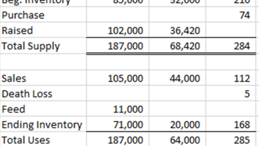
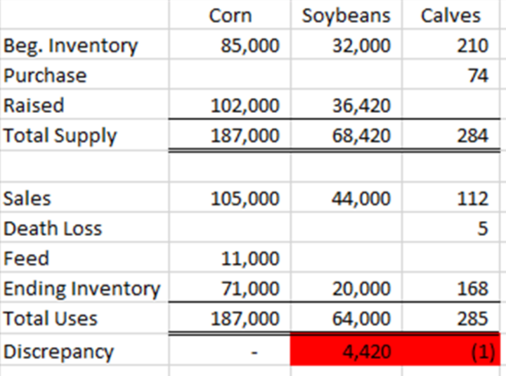
Using the example provide (Figure 1), we want Excel to notify us when an inventory reconciliation does not balance. To do this, first highlight the cells that calculate the discrepancy, if any, for each inventory category. In the home ribbon, about halfway over, you will notice a Conditional Formatting button that will provide a drop-down list. Once clicked you will see there are many preset options to choose from. For our example, we want to hover over Highlighted Cell Rules and then click on the last option which is More Rules. A pop-up box will appear. We want the discrepancy cell to visually cue us if the value is not zero. Select the rule: Format only cells that contain __. The preset option for the conditional calculation is greater than, but we will want to change it to not equal to, and then set the value in the third box to zero. To choose a color format that will display, click on format. Then select red from the Fill tab and click OK. With that rule in place anytime an inventory category has a discrepancy, it will display a red cell.

Conclusion

Conditional formatting is a quick tool that provides visual cues to draw attention to essential details in a spreadsheet. Finding trends and patterns will become much more straightforward as you begin to use this tool. Once you master the basics, you can start using data bars, color scales, and icons as well. If you’re using Excel to help manage your recordkeeping, learning to use more features can help make your life easier while creating a spreadsheet that’s a little more fun and user-friendly.